What Dirac's Delta Was Introduced For
A note on when and how the delta function was introduced, and on how Dirac himself describes it in the 1927 paper and in the 1930 book.
A few days ago, reading Weinberg’s The Quantum Theory of Fields with a group of colleagues, we spent some time on the delta function.
The image most of us carry is that of a normal curve — a Gaussian, for instance — made narrower and taller, with the area held at one, until in the limit it vanishes everywhere except at the origin.
Applied to quantum mechanics, the delta can represent the wave function of a quantum system: is the representation of the state in the basis . Read that way, and holding fixed while varies, the expression is a wave function concentrated at a single point, and the image then gives the particle localised at a point as an idealised limiting case.
In field theory the same symbol is usually met in another role: at each vertex of a Feynman diagram it expresses the conservation of four-momentum, and it is what forces the momenta entering the vertex to add up to the momenta leaving it.
That one mathematical object should take different interpretations in different contexts is unremarkable. It did, however, push me to ask what the symbol was introduced for, and whether it was then used for that purpose or for another. So I went to look at when and how it was introduced, and at how Dirac himself describes it in the two texts where he presents it, the 1927 paper and the 1930 book.
The Gaussian image turns out to belong to Kirchhoff, and to predate Dirac by forty-five years. In 1882, working on Green’s theorem in the study of Huygens’ principle, Kirchhoff defined an object he wrote , vanishing for all finite values of its argument, positive for infinitely small ones, and with unit integral; he justified the assumption by observing that a Gaussian with a large parameter approximates it. The setting is wave optics, and the object is there to make an integral over a surface produce the value of a field at a chosen instant: no states, no particles. Heaviside introduced the same object, or its equivalent, into electromagnetic theory about ten years later, in the course of his operational calculus for electric networks, and Paul Hertz used it in statistical mechanics in 1916.1
Dirac’s 1927 paper, The Physical Interpretation of the Quantum Dynamics, introduces the symbol in a section titled “Notation”.2 The reason given is that one cannot get far in a theory of matrices whose rows and columns run over continuous ranges without a notation of this kind. Where a matrix has discrete indices, the entries of the identity are given by the Kronecker delta, which is one when the two indices agree and zero otherwise; when the indices vary continuously, no ordinary function will do the same job, and this is the gap the new symbol fills. Dirac notes that the object is not a proper function of and can be regarded as the limit of a sequence of functions, and does not return to the remark. He then lists its properties — among them that the condition of vanishing away from the origin can be written as the algebraic equation — and states the use he needs it for: expressing the elements of the unit matrix. Jammer describes the same use, reconstructing Dirac’s application of the symbol to the elements of a continuous unit matrix and of a general continuous diagonal matrix.3
In the 1930 book the symbol arrives from a difficulty raised earlier. In §10 Dirac observes that the scalar product of eigenkets belonging to a continuous range of eigenvalues must be infinitely great if a certain integral is not to vanish, and he defers to §15 the form of infinity required.4 Eigenkets are states, so here the symbol enters a discussion in which states are already present; the task it performs is the normalisation of a continuous basis. The Gaussian picture appears in §15, with a clause worth noting: after describing a function that vanishes outside a small domain and whose integral over that domain is unity, Dirac adds that the exact shape of the function inside the domain does not matter, provided there are no unnecessarily wild variations. He then calls the object an “improper function” to mark its difference from a function in the usual sense, and remarks, a page later, that using improper functions involves no lack of rigour and amounts to a convenient notation — one could rewrite the relations without them, though only in a cumbersome way that would obscure the argument.
There is one further image, and it is the one Dirac attributed to himself. In a 1963 interview he said that all electrical engineers are familiar with the idea of a pulse, and that the delta function is “just a way of expressing a pulse mathematically”. He had trained as an electrical engineer at Bristol and had studied Heaviside’s operational calculus, and Jammer lists both among the things that contributed.5 The remark is retrospective, made nearly forty years after the fact, and what it describes is the pulse.
It is worth setting the two present-day uses side by side. In quantum mechanics, is the scalar product of two eigenkets of position, and says that it vanishes unless the two labels agree; fix one label and the same expression can be read as the wave function of that eigenket in the position basis, which is where the picture of a particle at a point comes from. In field theory, the delta at a vertex has momenta on both sides of its argument and no ket attached to either: it says that the total momentum entering agrees with the total momentum leaving, and its effect is to remove from the calculation every configuration in which they do not. In both cases the symbol asserts that two sets of labels coincide; what differs is whether one of those labels also names a state.
The image we carry, then, is a composite, and its parts come from different places. The Gaussian is Kirchhoff’s and belongs to wave optics; the reading in terms of a localised particle is later than both of Dirac’s presentations; and in both of them the symbol is introduced for the same purpose, which is to write down an identity — the unit matrix in 1927, the normalisation of a continuous basis in 1930.
One consequence is worth spelling out. When we say that describes a particle localised at a point, and add that this is an idealisation, the idealisation lies in the eigenket rather than in the delta. A state of perfectly definite position is not a state in the ordinary sense: it has infinite norm, it cannot be normalised to unit probability, and no physical preparation corresponds to it — which is why Dirac has to relax, in §10, the requirement that scalar products be finite. The delta is what one writes down once that relaxation has been made, in order to record that two such kets are orthogonal unless their labels agree. Taken by itself it is a piece of notation, and it says the same thing in field theory, where no improper state is involved at all.
Footnotes
-
M. Jammer, The Conceptual Development of Quantum Mechanics, pp. 316–317, which gives the references: G. Kirchhoff, “Zur Theorie der Lichtwellen”, Berliner Berichte 1882, pp. 641–669 (the passage is at p. 644), and Vorlesungen über mathematische Optik, Teubner 1891, vol. 2, pp. 24–25; O. Heaviside, “On operators in physical mathematics”, Proceedings of the Royal Society of London (A) 52 and 54, 1893; P. Hertz, “Statistische Mechanik”, 1916. ↩
-
P. A. M. Dirac, “The Physical Interpretation of the Quantum Dynamics”, Proceedings of the Royal Society of London (A) 113 (1927), 621–641; the delta is introduced in §2, pp. 625–627. ↩
-
Jammer, Conceptual Development, p. 317. ↩
-
P. A. M. Dirac, The Principles of Quantum Mechanics, 4th ed.; §10 at p. 39, §15 at pp. 58–59. ↩
-
Jammer, Conceptual Development, p. 316, citing an interview with Dirac of 14 May 1963 in the Archive for the History of Quantum Physics. ↩
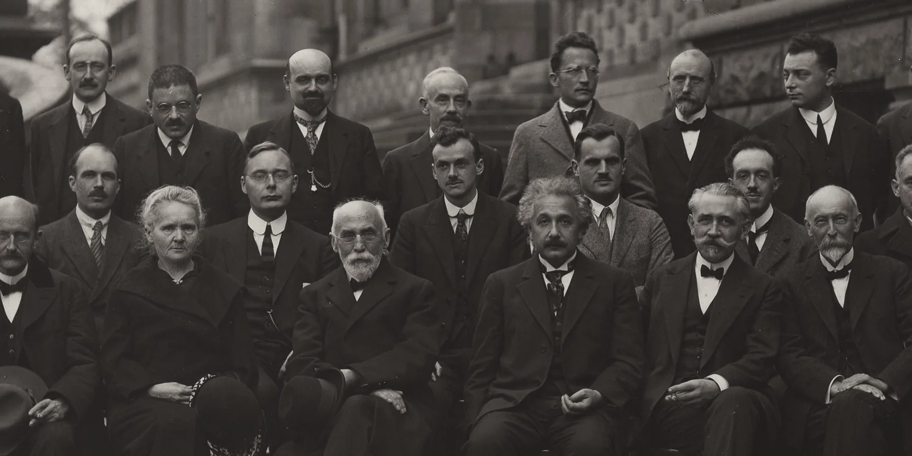
Header photograph: Benjamin Couprie, Solvay Conference 1927 — public domain, via Wikimedia Commons